head(classroom, 4) learner_id study_hours quiz_score
1 1 1 48
2 2 2 55
3 3 2 51
4 4 3 62Course 2 · About two hours of study
Prerequisites: Course 1 skills in running scripts, inspecting tables, calculating means, and reading a scatterplot. Previous regression training is unnecessary. This is Course 2, Module 2; it is not the next module after Course 1, Module 1.
How do study hours and quiz scores vary together in a small class? We will fit a straight line, use it to make two predictions, and explain the limits of the result. We are learning how to read a model, not trying to prove that additional studying causes a particular improvement.
By the end, you should be able to:
Download the complete local starter script. It includes the same 12 fictional classroom records as Course 1, Module 1, so it runs from any folder without data downloads or additional packages. Run it from the top in a fresh R session. The plot block runs when you use R interactively in an editor.
Our outcome is quiz_score, measured in points from 0 to 100. Our predictor is study_hours, measured in hours. A predictor is an input to the model; the word does not establish that it causes the outcome. One row is one fictional learner.
head(classroom, 4) learner_id study_hours quiz_score
1 1 1 48
2 2 2 55
3 3 2 51
4 4 3 62Before fitting anything, predict the direction of the relationship. Then run this plot code in your editor:
plot(classroom$study_hours, classroom$quiz_score)Pair activity, ten minutes: describe the direction, identify two learners with the same study hours but different scores, and explain why a single line will not pass through every point. At four hours the two scores are 68 and 63, already showing variation that study time alone does not describe.
A simple linear regression describes the outcome with an intercept and a slope. The intercept sets the line’s level at zero hours. The slope describes how much the predicted score differs when study time differs by one hour. R chooses the line that minimizes the sum of squared vertical differences between observed and fitted scores.
score_model <- lm(quiz_score ~ study_hours, data = classroom)
coef(score_model)
(Intercept) study_hours
40.736842 6.315789 Read the formula from left to right: quiz_score is the outcome; ~ separates it from the predictor; study_hours is the predictor. data = classroom tells R which table holds those columns. <- saves the fitted model under the name score_model. coef() displays its coefficients.
The fitted relationship is approximately:
Predicted score = 40.74 + 6.32 × study hours.
One more study hour is associated with about 6.32 more predicted score points in these constructed records. The intercept, about 40.74, is the fitted value at zero hours. No observation has zero study hours, so we should not describe it as an observed zero-hour score.
Guided practice, ten minutes: point to the outcome, predictor, and dataset in the formula. Explain which part you would change to use a different table and which part you would change to model a different outcome. Do not add new variables yet.
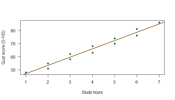
The points are observed scores; the line shows fitted scores. A learner can lie above or below it. The vertical difference between an observed and fitted score is called a residual. Residuals remind us that a model is a summary rather than a complete description of every case.
Discuss: if all points were exactly on this line, would that alone prove a causal effect? Explain why a perfect description of these records would still say nothing about how they were generated or what an intervention would do.
Before running the next code, predict which fitted score is larger and by how much. newdata supplies the predictor values for which we want predictions; its column name must match the model’s predictor.
predict(score_model, newdata = data.frame(study_hours = c(3, 4))) 1 2
59.68421 66.00000 The predicted scores are approximately 59.68 at three hours and 66 at four hours. The difference is about 6.32 points, matching the slope. The original scores at four hours were 68 and 63, not exactly 66.
Hands-on, ten minutes: predict scores at two and five hours. Explain the difference between a fitted prediction and an observed score. Then consider a prediction at 20 hours: it lies far outside the observed range of one to seven hours, so extending this straight line there would require an unsupported assumption.
A fitted line summarizes an association conditional on the variables and records we gave it. It does not establish why that pattern exists. In a real study, earlier preparation might influence both study time and quiz results. Students could also choose study time in response to their expected difficulty.
Here, the data are explicitly fictional. A small standard error or a low p-value would not turn them into evidence about actual students. Our aim is to practice code and interpretation. A later causal-inference module asks what additional design and assumptions a causal question requires.
If you see object 'quiz_score' not found, check names(classroom) and the data argument. If prediction reports that study_hours is missing, check the column name in newdata. If the script works only after other code has run, restart R and execute the downloaded script from its first line.
Allow 20 minutes. Work with the supplied records without changing their values.
study_hours <= 5. Before running it, predict whether the slope must stay identical.Use predict(score_model, newdata = data.frame(study_hours = 5)). A filtered base R table can be written as classroom[classroom$study_hours <= 5, ]; the blank after the comma retains every column. Keep the full-sample model under its original name.
predict(score_model, newdata = data.frame(study_hours = 5)) 1
72.31579 score_model_small <- lm(
quiz_score ~ study_hours,
data = classroom[classroom$study_hours <= 5, ]
)
coef(score_model_small)(Intercept) study_hours
41.321429 6.107143 The prediction is about 72.32 points. The restricted slope is about 6.11 points per hour, rather than 6.32. Changing the sample need not preserve the fitted coefficients. Neither fit is an empirical finding about a real population.
A suitable interpretation is: “In the fictional classroom records, an additional reported study hour is associated with about 6.32 more predicted score points. These constructed observations do not establish a causal effect or describe a real population.”
The formula specifies a question, the fitted line summarizes a relationship, and a prediction gives a value on that line. Always retain the units, inspect the observations, and distinguish a description from a causal claim.
Exit question: a classmate says, “R predicts 66 points at four hours, so giving everyone four hours of study guarantees 66.” Explain two different problems with that sentence.
For homework, save your modified script and a short interpretation. A dedicated regression chapter in the textbook is planned; this pilot contains the explanations needed for its own activities.