study_hours <- 3
study_hours
[1] 3study_hours + 1[1] 4The same material as the module views, gathered into one continuous view. Only two modules are authored pilots; planned modules retain their existing curriculum descriptions.
Section numbers identify the course and module: 2.2 corresponds to Course 2, Module 2.
Data preparation › Module 1
Course 1, Module 1 · Open module view
Course 1 · About two hours of study · No prior R required
This lesson uses 12 fictional classroom records. It requires R and an editor, but no extra packages, accounts, or data downloads. Nothing in these records supports a claim about real learners.
How can we describe study time and quiz scores in a small class? Today you will run a saved script, inspect a table, and explain one summary. You do not need to memorize the commands. The aim is to know what each line asks R to do and how to check its result.
By the end, you should be able to:
Before class, install R and RStudio Desktop. An existing Positron or VS Code setup is also suitable. We demonstrate RStudio to keep the first module consistent. An optional coding assistant is unnecessary for this lesson.
Download the complete starter script. Save it in a folder called r4ss-course and open it in your editor. The script constructs its own small dataset, so its location does not affect whether it runs.
In RStudio, the source editor holds the script you save. The console receives commands and displays results. Put the cursor on a line, then press Ctrl+Enter on Windows or Cmd+Enter on macOS. Run from the top in order. The text beginning with # is a comment for the reader.
A leading > is the console prompt; do not type it into your script. If the console shows +, R may be waiting for a closing parenthesis or quotation mark. Press Esc, check the line, and run the complete expression again. Save the script with Ctrl+S or Cmd+S.
Check whether R itself opens, then whether your editor can find it. Ask for help with the exact error message. While troubleshooting, use the rendered outputs below to make predictions and complete the interpretation questions with a partner.
Read the next three lines before running them. <- stores a value under a name. Writing that name asks R to display its value. Adding one calculates a result.
study_hours <- 3
study_hours[1] 3study_hours + 1[1] 4The result of the addition is 4. The object still stores 3 because the addition did not assign a replacement value. You can check by running study_hours again.
Hands-on, five minutes: change the assigned value to 5, run all three lines again, and explain the two displayed results to a partner. Then restore 3 so the rest of the lesson matches this page.
A dataset is often organized as a table. Here, learner_id identifies a person, study_hours records reported study time in hours, and quiz_score records a score from 0 to 100. These names are case-sensitive. The three columns describe different properties of the same people.
Run this block once. c() collects several values, and data.frame() arranges equal-length columns into a table. You can reuse this supplied block without learning every detail today.
# Fictional classroom records, created solely for these lessons.
classroom <- data.frame(
  learner_id = 1:12,
  study_hours = c(1, 2, 2, 3, 3, 4, 4, 5, 5, 6, 6, 7),
  quiz_score = c(48, 55, 51, 62, 58, 68, 63, 74, 70, 81, 76, 86)
)
Now inspect the beginning and count the rows:
head(classroom, 3) learner_id study_hours quiz_score
1 1 1 48
2 2 2 55
3 3 2 51nrow(classroom)[1] 12head(classroom, 3) displays the first three rows. It does not remove the remaining records. nrow() counts all 12 rows. The row numbers printed at the left help display the table; learner_id is our explicit identifier column.
Hands-on, ten minutes: display the first five rows instead. Explain why this changes the display but not the result of nrow(classroom). Find the score of learner 3 by reading the printed table. Do not change the data yet.
The $ symbol selects a named column from a table. classroom$quiz_score means the quiz_score column in classroom. The function mean() takes numeric values and calculates their arithmetic mean.
mean(classroom$study_hours)[1] 4mean(classroom$quiz_score)[1] 66The average reported study time is 4 hours, and the average score is 66 points. Neither statement says that everyone has that value. These are descriptions of these 12 fictional records only. There are no missing values in this example; a later module explains how missing values affect summaries.
Discuss: what information disappears when we replace the 12 scores with just one mean? Compare the smallest and largest displayed scores before answering.
extra_hour <- study_hours + 1
extra_hour
[1] 4study_hours[1] 3extra_hour stores a new value of 4, while study_hours remains 3. An object and a column can have related names, but study_hours and classroom$study_hours are different expressions. Changing the single object does not change the table column.
If you see object 'classroom' not found, run the data-creation block first. If a function returns NA with a warning, read that warning and check the input; repeated clicks rarely fix a misspelled column. Use names(classroom) to inspect the actual names.
Allow 15 minutes. Save a copy of the starter script with your name in the filename.
planned_hours with value 6. Calculate planned_hours + 2 without replacing it. Display planned_hours again.classroom and count all its rows.planned_hours would not change the class mean.Reuse the assignment pattern, head(), nrow(), and mean() above. A comment begins with #. Check the object name and column capitalization before looking at the solution.
planned_hours <- 6
planned_hours + 2
planned_hours
head(classroom, 4)
nrow(classroom)
mean(classroom$quiz_score)
# The mean quiz score is 66 points across 12 fictional learners.
The first calculation displays 8; planned_hours still displays 6. There are 12 rows. The separate object does not alter a column in classroom.
A script stores instructions; the console runs them and shows results. Assignment stores a value, a table organizes observations, and a summary describes a set of values. Save your script, restart R, and run it from the top to check that it works without objects left over from earlier attempts.
Exit question: explain the difference between study_hours, classroom$study_hours, and mean(classroom$study_hours) in your own words.
Before moving to the next module, write two sentences describing what you can infer from the mean and what you cannot. The textbook reading is Introduction to R; its wider discussion of data structures is optional at this stage.
Data preparation › Module 2
Course 1, Module 2 · Open module view
Course 1 · About two hours of study
This page contains the existing curriculum description, not an authored lesson.
Identify observations, variables, types, and import settings.
Import a CSV and compare its rows and column types with the source.
Data preparation › Module 3
Course 1, Module 3 · Open module view
Course 1 · About two hours of study
This page contains the existing curriculum description, not an authored lesson.
Distinguish selecting columns, filtering rows, and ordering observations.
Select variables, filter observations, and sort the resulting table.
Data preparation › Module 4
Course 1, Module 4 · Open module view
Course 1 · About two hours of study
This page contains the existing curriculum description, not an authored lesson.
Read a pipeline and construct variables with explicit definitions.
Build a short pipeline that creates a variable and checks its values.
Data preparation › Module 5
Course 1, Module 5 · Open module view
Course 1 · About two hours of study
This page contains the existing curriculum description, not an authored lesson.
Recode values and distinguish missing-value definitions.
Recode a category, mark missing codes, and compare valid counts.
Data preparation › Module 6
Course 1, Module 6 · Open module view
Course 1 · About two hours of study
This page contains the existing curriculum description, not an authored lesson.
Choose grouped summaries and state percentage denominators.
Produce group counts, means, and percentages with explicit denominators.
Data preparation › Module 7
Course 1, Module 7 · Open module view
Course 1 · About two hours of study
This page contains the existing curriculum description, not an authored lesson.
Match ggplot2 plots to distributions and group comparisons.
Plot a distribution and group comparison, then inspect unusual values.
Data preparation › Module 8
Course 1, Module 8 · Open module view
Course 1 · About two hours of study
This page contains the existing curriculum description, not an authored lesson.
Identify join keys and anticipate unmatched or repeated records.
Join two tables and audit unmatched keys and row counts.
Data preparation › Module 9
Course 1, Module 9 · Open module view
Course 1 · About two hours of study
This page contains the existing curriculum description, not an authored lesson.
Recognize how reshaping changes table structure and observation keys.
Reshape a table between long and wide forms and verify identifiers.
Data preparation › Module 10
Course 1, Module 10 · Open module view
Course 1 · About two hours of study
This page contains the existing curriculum description, not an authored lesson.
Clean strings and parse dates while checking failed conversions.
Standardize text labels and convert a date field with checks.
Data preparation › Module 11
Course 1, Module 11 · Open module view
Course 1 · About two hours of study
This page contains the existing curriculum description, not an authored lesson.
Locate and repair errors across a data-preparation workflow.
Audit and repair a workflow combining cleaning, joins, and summaries.
Data preparation › Module 12
Course 1, Module 12 · Open module view
Course 1 · About two hours of study
This page contains the existing curriculum description, not an authored lesson.
Turn raw records into an analysis-ready dataset with documented checks.
Prepare a dataset and explain the main cleaning and transformation choices.
Regression › Module 1
Course 2, Module 1 · Open module view
Course 2 · About two hours of study
This page contains the existing curriculum description, not an authored lesson.
Connect research questions, variables, statistical summaries, and uncertainty.
Identify an outcome, predictors, and the uncertainty in a proposed comparison.
Regression › Module 2
Course 2, Module 2 · Open module view
Course 2 · About two hours of study
Prerequisites: Course 1 skills in running scripts, inspecting tables, calculating means, and reading a scatterplot. Previous regression training is unnecessary. This is Course 2, Module 2; it is not the next module after Course 1, Module 1.
How do study hours and quiz scores vary together in a small class? We will fit a straight line, use it to make two predictions, and explain the limits of the result. We are learning how to read a model, not trying to prove that additional studying causes a particular improvement.
By the end, you should be able to:
Download the complete local starter script. It includes the same 12 fictional classroom records as Course 1, Module 1, so it runs from any folder without data downloads or additional packages. Run it from the top in a fresh R session. The plot block runs when you use R interactively in an editor.
Our outcome is quiz_score, measured in points from 0 to 100. Our predictor is study_hours, measured in hours. A predictor is an input to the model; the word does not establish that it causes the outcome. One row is one fictional learner.
head(classroom, 4) learner_id study_hours quiz_score
1 1 1 48
2 2 2 55
3 3 2 51
4 4 3 62Before fitting anything, predict the direction of the relationship. Then run this plot code in your editor:
plot(classroom$study_hours, classroom$quiz_score)Pair activity, ten minutes: describe the direction, identify two learners with the same study hours but different scores, and explain why a single line will not pass through every point. At four hours the two scores are 68 and 63, already showing variation that study time alone does not describe.
A simple linear regression describes the outcome with an intercept and a slope. The intercept sets the line’s level at zero hours. The slope describes how much the predicted score differs when study time differs by one hour. R chooses the line that minimizes the sum of squared vertical differences between observed and fitted scores.
score_model <- lm(quiz_score ~ study_hours, data = classroom)
coef(score_model)
(Intercept) study_hours
40.736842 6.315789 Read the formula from left to right: quiz_score is the outcome; ~ separates it from the predictor; study_hours is the predictor. data = classroom tells R which table holds those columns. <- saves the fitted model under the name score_model. coef() displays its coefficients.
The fitted relationship is approximately:
Predicted score = 40.74 + 6.32 × study hours.
One more study hour is associated with about 6.32 more predicted score points in these constructed records. The intercept, about 40.74, is the fitted value at zero hours. No observation has zero study hours, so we should not describe it as an observed zero-hour score.
Guided practice, ten minutes: point to the outcome, predictor, and dataset in the formula. Explain which part you would change to use a different table and which part you would change to model a different outcome. Do not add new variables yet.
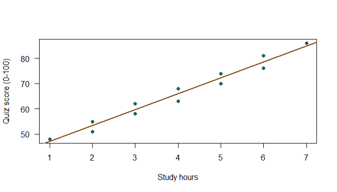
The points are observed scores; the line shows fitted scores. A learner can lie above or below it. The vertical difference between an observed and fitted score is called a residual. Residuals remind us that a model is a summary rather than a complete description of every case.
Discuss: if all points were exactly on this line, would that alone prove a causal effect? Explain why a perfect description of these records would still say nothing about how they were generated or what an intervention would do.
Before running the next code, predict which fitted score is larger and by how much. newdata supplies the predictor values for which we want predictions; its column name must match the model’s predictor.
predict(score_model, newdata = data.frame(study_hours = c(3, 4))) 1 2
59.68421 66.00000 The predicted scores are approximately 59.68 at three hours and 66 at four hours. The difference is about 6.32 points, matching the slope. The original scores at four hours were 68 and 63, not exactly 66.
Hands-on, ten minutes: predict scores at two and five hours. Explain the difference between a fitted prediction and an observed score. Then consider a prediction at 20 hours: it lies far outside the observed range of one to seven hours, so extending this straight line there would require an unsupported assumption.
A fitted line summarizes an association conditional on the variables and records we gave it. It does not establish why that pattern exists. In a real study, earlier preparation might influence both study time and quiz results. Students could also choose study time in response to their expected difficulty.
Here, the data are explicitly fictional. A small standard error or a low p-value would not turn them into evidence about actual students. Our aim is to practice code and interpretation. A later causal-inference module asks what additional design and assumptions a causal question requires.
If you see object 'quiz_score' not found, check names(classroom) and the data argument. If prediction reports that study_hours is missing, check the column name in newdata. If the script works only after other code has run, restart R and execute the downloaded script from its first line.
Allow 20 minutes. Work with the supplied records without changing their values.
study_hours <= 5. Before running it, predict whether the slope must stay identical.Use predict(score_model, newdata = data.frame(study_hours = 5)). A filtered base R table can be written as classroom[classroom$study_hours <= 5, ]; the blank after the comma retains every column. Keep the full-sample model under its original name.
predict(score_model, newdata = data.frame(study_hours = 5)) 1
72.31579 score_model_small <- lm(
quiz_score ~ study_hours,
data = classroom[classroom$study_hours <= 5, ]
)
coef(score_model_small)(Intercept) study_hours
41.321429 6.107143 The prediction is about 72.32 points. The restricted slope is about 6.11 points per hour, rather than 6.32. Changing the sample need not preserve the fitted coefficients. Neither fit is an empirical finding about a real population.
A suitable interpretation is: “In the fictional classroom records, an additional reported study hour is associated with about 6.32 more predicted score points. These constructed observations do not establish a causal effect or describe a real population.”
The formula specifies a question, the fitted line summarizes a relationship, and a prediction gives a value on that line. Always retain the units, inspect the observations, and distinguish a description from a causal claim.
Exit question: a classmate says, “R predicts 66 points at four hours, so giving everyone four hours of study guarantees 66.” Explain two different problems with that sentence.
For homework, save your modified script and a short interpretation. A dedicated regression chapter in the textbook is planned; this pilot contains the explanations needed for its own activities.
Regression › Module 3
Course 2, Module 3 · Open module view
Course 2 · About two hours of study
This page contains the existing curriculum description, not an authored lesson.
Interpret reference categories and relationships conditional on another variable.
Compare predicted outcomes across categories and an interaction.
Regression › Module 4
Course 2, Module 4 · Open module view
Course 2 · About two hours of study
This page contains the existing curriculum description, not an authored lesson.
Assess functional form, residual patterns, and influential observations.
Inspect model diagnostics and explain a justified specification change.
Regression › Module 5
Course 2, Module 5 · Open module view
Course 2 · About two hours of study
This page contains the existing curriculum description, not an authored lesson.
Relate binary outcomes to logit/probit models and predicted probabilities.
Fit binary-outcome models and compare predicted probabilities.
Regression › Module 6
Course 2, Module 6 · Open module view
Course 2 · About two hours of study
This page contains the existing curriculum description, not an authored lesson.
Translate nonlinear model results into probabilities and marginal effects.
Calculate predictions or marginal effects for substantively meaningful profiles.
Regression › Module 7
Course 2, Module 7 · Open module view
Course 2 · About two hours of study
This page contains the existing curriculum description, not an authored lesson.
Distinguish ordered and unordered categorical outcomes and model assumptions.
Choose an ordinal or multinomial model and interpret category probabilities.
Regression › Module 8
Course 2, Module 8 · Open module view
Course 2 · About two hours of study
This page contains the existing curriculum description, not an authored lesson.
Represent choice sets and interpret alternative-specific predictors.
Arrange choice data and interpret a conditional-logit comparison.
Regression › Module 9
Course 2, Module 9 · Open module view
Course 2 · About two hours of study
This page contains the existing curriculum description, not an authored lesson.
Explain within-unit comparisons and unit/time fixed effects in panel data.
Compare pooled and fixed-effects estimates and state the identifying variation.
Regression › Module 10
Course 2, Module 10 · Open module view
Course 2 · About two hours of study
This page contains the existing curriculum description, not an authored lesson.
Distinguish within-group and between-group variation in hierarchical data.
Fit or inspect a multilevel model and interpret group variation.
Regression › Module 11
Course 2, Module 11 · Open module view
Course 2 · About two hours of study
This page contains the existing curriculum description, not an authored lesson.
Present regression estimates and predictions with clear substantive interpretation.
Prepare a regression table and plot with units, uncertainty, and a conclusion.
Regression › Module 12
Course 2, Module 12 · Open module view
Course 2 · About two hours of study
This page contains the existing curriculum description, not an authored lesson.
Choose and assess a regression model for a bounded research question.
Complete a model-based analysis with diagnostics and substantive interpretation.
Computational social science › Module 1
Course 3, Module 1 · Open module view
Course 3 · About two hours of study
This page contains the existing curriculum description, not an authored lesson.
Distinguish causal estimands, identification assumptions, and regression associations.
Specify a causal question and explain the comparison and assumptions it requires.
Computational social science › Module 2
Course 3, Module 2 · Open module view
Course 3 · About two hours of study
This page contains the existing curriculum description, not an authored lesson.
Use repeated simulation to examine sampling variation and estimator behavior.
Run a Monte Carlo experiment and explain how results change with sample size.
Computational social science › Module 3
Course 3, Module 3 · Open module view
Course 3 · About two hours of study
This page contains the existing curriculum description, not an authored lesson.
Connect agent rules and interactions to emergent social patterns.
Modify an agent rule and compare simulated aggregate patterns.
Computational social science › Module 4
Course 3, Module 4 · Open module view
Course 3 · About two hours of study
This page contains the existing curriculum description, not an authored lesson.
Connect priors, likelihood, posterior computation, and model checking.
Specify a simple Bayesian model and inspect posterior summaries and checks.
Computational social science › Module 5
Course 3, Module 5 · Open module view
Course 3 · About two hours of study
This page contains the existing curriculum description, not an authored lesson.
Distinguish model training, tuning, and evaluation on held-out data.
Compare predictive models using a consistent held-out evaluation.
Computational social science › Module 6
Course 3, Module 6 · Open module view
Course 3 · About two hours of study
This page contains the existing curriculum description, not an authored lesson.
Explain causal-effect estimation using nuisance models, orthogonal scores, and cross-fitting.
Identify nuisance predictions and cross-fitting steps in a causal-estimation workflow.
Computational social science › Module 7
Course 3, Module 7 · Open module view
Course 3 · About two hours of study
This page contains the existing curriculum description, not an authored lesson.
Interpret feature contributions to predictions and distinguish explanations from causal effects.
Read local and global SHAP summaries and state an interpretive limitation.
Computational social science › Module 8
Course 3, Module 8 · Open module view
Course 3 · About two hours of study
This page contains the existing curriculum description, not an authored lesson.
Explain how preprocessing and representation affect text-based measurements.
Compare two text representations and discuss their implications for a research question.
Computational social science › Module 9
Course 3, Module 9 · Open module view
Course 3 · About two hours of study
This page contains the existing curriculum description, not an authored lesson.
Assess image-derived social measures and their validity and limitations.
Evaluate an image-derived measure against the social concept it is intended to capture.
Computational social science › Module 10
Course 3, Module 10 · Open module view
Course 3 · About two hours of study
This page contains the existing curriculum description, not an authored lesson.
Connect coordinates, geographic units, spatial patterns, and social questions.
Map a social measure and discuss scale and spatial interpretation.
Computational social science › Module 11
Course 3, Module 11 · Open module view
Course 3 · About two hours of study
This page contains the existing curriculum description, not an authored lesson.
Distinguish relations, node attributes, network structure, and network summaries.
Construct or inspect a network and interpret a structural summary.
Computational social science › Module 12
Course 3, Module 12 · Open module view
Course 3 · About two hours of study
This page contains the existing curriculum description, not an authored lesson.
Match a computational method and validation strategy to a social research question.
Complete a bounded computational analysis and discuss measurement and inferential limits.
Programming › Module 1
Course 4, Module 1 · Open module view
Course 4 · About two hours of study
This page contains the existing curriculum description, not an authored lesson.
Write functions with clear inputs, outputs, and reusable responsibilities.
Turn repeated code into a function and check it on different inputs.
Programming › Module 2
Course 4, Module 2 · Open module view
Course 4 · About two hours of study
This page contains the existing curriculum description, not an authored lesson.
Use conditions and iteration to automate repeated research tasks.
Automate a repeated task and handle a failed input explicitly.
Programming › Module 3
Course 4, Module 3 · Open module view
Course 4 · About two hours of study
This page contains the existing curriculum description, not an authored lesson.
Distinguish document structure, extractable text, and scanned pages.
Extract text or tables from a document and check the result against the source.
Programming › Module 4
Course 4, Module 4 · Open module view
Course 4 · About two hours of study
This page contains the existing curriculum description, not an authored lesson.
Work with image representations, processing, OCR, and extraction errors.
Inspect an image-processing or OCR workflow and verify its output.
Programming › Module 5
Course 4, Module 5 · Open module view
Course 4 · About two hours of study
This page contains the existing curriculum description, not an authored lesson.
Use interactive controls to explore and communicate plotted data.
Create or modify an interactive plot and assess its usability.
Programming › Module 6
Course 4, Module 6 · Open module view
Course 4 · About two hours of study
This page contains the existing curriculum description, not an authored lesson.
Organize related outputs into a coherent research dashboard.
Assemble a dashboard with a clear question, views, and navigation.
Programming › Module 7
Course 4, Module 7 · Open module view
Course 4 · About two hours of study
This page contains the existing curriculum description, not an authored lesson.
Choose selective reading, deferred computation, and suitable data workflows.
Process a larger dataset while explaining memory and computation choices.
Programming › Module 8
Course 4, Module 8 · Open module view
Course 4 · About two hours of study
This page contains the existing curriculum description, not an authored lesson.
Assess numerical approximation, optimization, precision, and convergence.
Compare numerical approximations or optimizers and inspect convergence and error.
Programming › Module 9
Course 4, Module 9 · Open module view
Course 4 · About two hours of study
This page contains the existing curriculum description, not an authored lesson.
Distinguish algorithmic improvements from compiled-code acceleration.
Compare an R workflow with a demonstrated compiled implementation and verify results.
Programming › Module 10
Course 4, Module 10 · Open module view
Course 4 · About two hours of study
This page contains the existing curriculum description, not an authored lesson.
Connect R workflows to language-model inputs, structured outputs, and validation.
Design an LLM-assisted task with explicit output checks and failure handling.
Programming › Module 11
Course 4, Module 11 · Open module view
Course 4 · About two hours of study
This page contains the existing curriculum description, not an authored lesson.
Specify research requirements and review code, deliverables, and interfaces.
Write a task specification with inputs, expected outputs, and acceptance checks.
Programming › Module 12
Course 4, Module 12 · Open module view
Course 4 · About two hours of study
This page contains the existing curriculum description, not an authored lesson.
Integrate reusable code and computational tools into a research workflow.
Develop a small workflow with documented interfaces, outputs, and checks.